The unreasonable effectiveness of volatility targeting - and where it falls short

Part 1: Introduction, a paradox & blindspots

This is part 1 of our in-depth investigation of how quantitative risk management could help improve risk-adjusted returns: I'll explain what volatility targeting is, explore a seemingly paradoxical phenomenon, and highlight its blindspots.

Volatility targeting’s goal is to keep an asset or portfolio’s volatility within reasonable boundaries, by actively adjusting exposure - it’s among the very few effective, universal techniques in quantitative finance. I can’t really think of many other than “diversification” and volatility targeting, if I had to answer on the spot.

A quick intro: inverse volatility scaling means when an asset is getting more volatile, you should reduce your exposure to it. People usually measure volatility with a rolling standard deviation of an asset’s returns. It looks usually something like this:

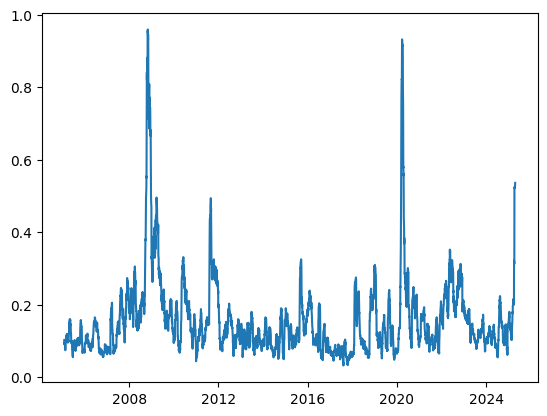
Volatility usually clusters — when the markets are volatile, they stay volatile for some time. You can kind of see it on the chart above, it doesn’t go “go back immediately” to its starting position¹. But, it does mean revert after some time.

Volatility targeting is using inverse volatility scaling with a pre-defined (annualized) volatility target level. The S&P500’s annualized volatility is around 16%, Bitcoin’s is around 60%.

You can make your strategy, or asset’s cumulative returns comparable by using the same volatility target on them. It’s also a good way to normalize the risk contribution of each asset within a portfolio - so a really volatile asset won’t dominate it.

What’s the opposite of volatility targeting?

I’d say “buying the dip” is a pretty good contender - as inverse volatility scaling can be translated into: “reducing your exposure on a dip”.

And buying the dip is also effective. I think fundamentally almost all systematic strategies that trade the SP500 only a couple times per year, long-only, are quantitative equivalent of “buying-the-dip” (and ideally should be called as such, for transparency reasons). Retail investors kind of intuitively understand its effectiveness.

If you plot the average 30 day forward returns when the SP500 was in a drawdown, you’d see this²:

The higher the drawdown, the larger the 30 day forward returns (SPY). Check footnote for the caveat with these plots.

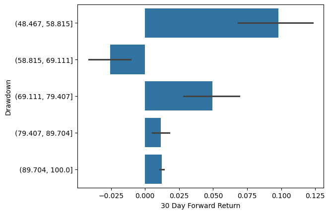
This chart indicates that you should have bought the most when SP500 is in the biggest drawdown — thank you for that, captain hindsight! Of course this is not something that can be effectively executed, and definitely can not be called a risk management technique.

There are fundamental differences here that makes this comparison impossible: buy-the-dip assumes you have cash to allocate, while volatility targeting assumes that you are fully invested (calculated based on the current volatility level).

Although you could add to a position if it gets volatile (which usually means its price is falling), that’d would be more of “buy more when in drawdown” technique. But that sounds pretty dangerous, kind of the opposite of a risk management strategy.

The paradox

We looked at what the average returns were when the SP500 was in different drawdowns. Let’s look at what they are when volatility is in a certain range³:

The higher the annualized volatility, the higher the returns - as well as there’s a massive increase in volatility as well. Check footnote for the caveat with these plots.

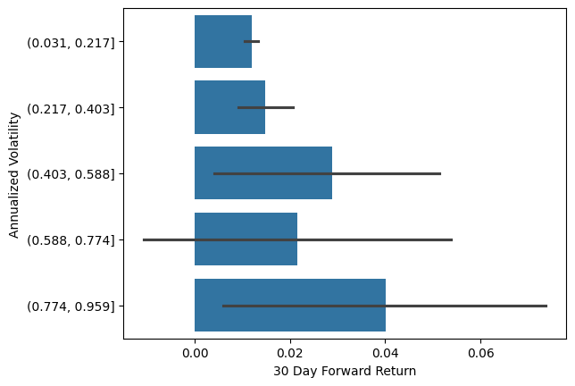
When volatility was really high, we get higher average forward returns, than in the low volatility regime - there’s a catch of course. But that’s the opposite of what we’re looking for!

Let’s look at the simplest possible backtest we could create, where we use volatility targeting with a 20 day rolling window on the SP500, rebalancing daily, with fixed 0.1% transaction costs:

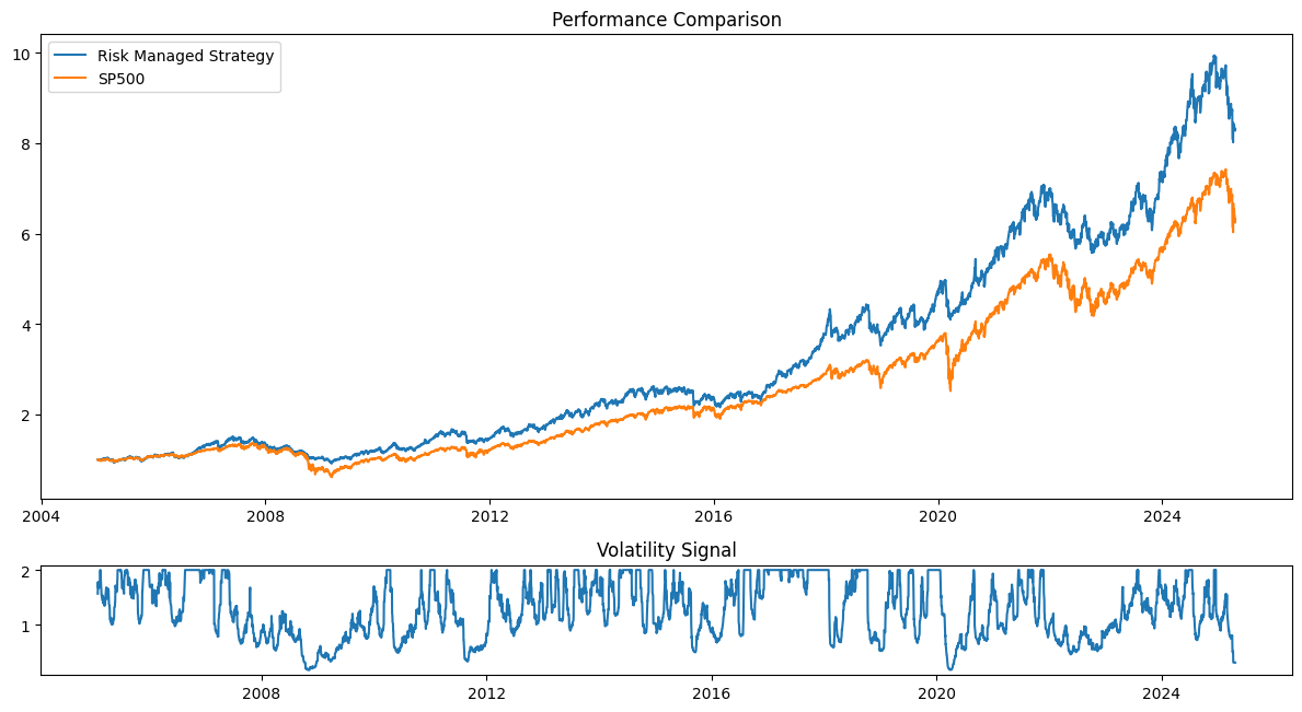
You usually get 10-20% increase in risk-adjusted returns when you “blindly”⁴ apply volatility targeting on an asset.⁵

How is this possible? How come

It’s mainly because of “volatility drag” - the difference between cumulative average returns (a multiplicative process) and average returns (an additive process). We could mitigate its effect by averaging log returns instead of arithmetic returns, per Kris’ explanation.

Try it yourself

We released a small python package (with MIT Licence) that helps you apply volatility targeting on any return series.

It’s a collection of transparent, easy-to-audit functions, that we wrapped it into a package called risklab on pypi — it’s super easy to use:

vol_signal = scale_to_target_volatility(
    target_volatility=0.16, # the annualized volatility target
    rolling_window=20,
    returns=sp500_data["Close"].pct_change(),
    upper_limit=2.0,
    lag=0,
    fill_initial_period_with_mean=False,
    annualization_period=252,
)
results = backtest_signal(
    signal=vol_signal,
    underlying=sp500_data["Close"].pct_change(),
    transaction_cost=0.001,
    lag=0,
)

Explore what asset classes volatility targeting works best for using risklab and this notebook.

Is this a silver bullet? What am I missing?

I personally always felt a bit cautious using only past volatility to manage risk. It basically means you’re over-leveraged at times when volatility is very low, to compensate for reduced leverage when its high. Looks fine in a backtest, but it’s a lot more uncomfortable when you are actually trading.

The missing piece is the realization that:

not all periods of very low volatility are created equal.

Unexpected events may hit when:

• Volume, liquidity is structurally low

• Implied volatility and the volatility risk premium is low

• Leverage is high

In those cases, you probably see massive moves, “de-leveraging” events where people have to reduce their exposure. Some may call it “Risk parity sell-of” or “Carry trade unwinds” - and their effect are probably exaggerated by the widespread usage of volatility-based risk management itself!

Last summer, implied & realized volatility were all at the lowest points in the last couple of years. VIX term structure was extremely flat, volumes were low (usual summer break vibes) — all of these were signs that a small sell-off could trigger a lot bigger one.

Can we use these and similar, asset-specific, or market-wide risk factors to reduce the harm of the sudden de-leveraging events, like August 2024? I believe so — you can explore them for crypto here, and will cover more assets soon.

We work on Unravel, where we make forward-looking, exogenous risk factors available and easy-to-use - starting with the most volatile assets.

As always, happy to connect on LinkedIn or X.

This is part 1 of an in-depth investigation of how quantitative risk management could help improve risk-adjusted returns. We’ll cover the mechanics, the implementation details, benchmark the different “risk proxies”, ensembling and a lot more!

1. Although there’s definitely an artifact here: the rolling window calculation.

2. These factor plots are misleading, as they’re using equal bin size, and the number of observations in each bin are very skewed - the market is mainly in a low-volatile state.

3. These factor plots are misleading, as they’re using equal bin size, and the number of observations in each bin are very skewed - the market is mainly in a low-volatile state.

4. “Blindly” in this case does mean using a 20 day lookback window, coming from reasonable priors, but there’s always a chance that this is overfitting already.

5. Although it didn’t perform particularly well in equities after 2008!